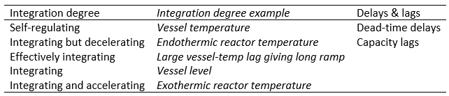
Process response depends on process variable’s self-regulation
An indication of the ease with which a process may be controlled can be obtained by plotting the process reaction curve. This curve is constructed after having first stabilized the process temperature under manual control and then making a nominal change in heat input to the process, such as 10%. A temperature recorder then can be used to plot the temperature versus time curve of this change.[1]
Process response of self-regulating process variable vs. time:
vessel temperature after heating increase
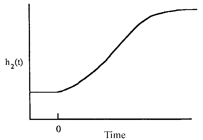
Process response of integrating process variable vs. time:
vessel level after inflow increase [2]
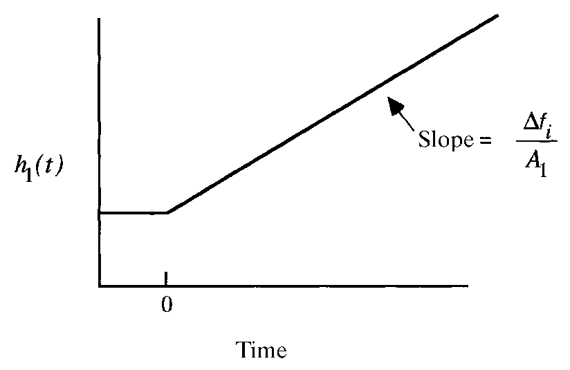
Another phenomenon associated with a process or system is identified as the steady-state transfer-function characteristic. Since many processes are nonlinear, equal increments of heat input do not necessarily produce equal increments in temperature rise. The characteristic transfer-function curve for a process is generated by plotting temperature against heat input under constant heat input conditions. Each point on the curve represents the temperature under stabilized conditions, as opposed to the reaction curve, which represents the temperature under dynamic conditions. For most processes this will not be a straight-line, or linear, function.
Temperature gain vs. heat input of endothermic process:
heating a liquid till it boils and absorbs more heat
As the temperature increases, the slope of the tangent line to the curve has a tendency to decrease. This usually occurs because of increased losses through convection and radiation as the temperature increases. This process gain at any temperature is the slope of the transfer function at that temperature. A steep slope (high ΔT/ΔH) is a high gain; a low slope (low ΔT/ΔH) is a low gain.
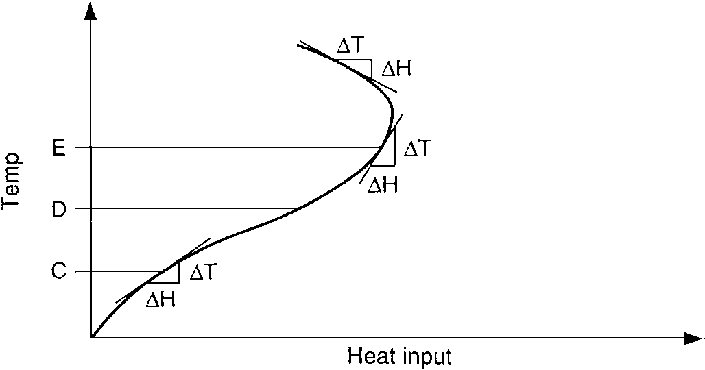
Temperature gain vs. heat input of exothermic process:
heating a mixture of reactants till their reaction gives off reaction heat;
melting a plastic till its flow gives off frictional heat
This curve follows the endothermic curve up to the temperature level D. At this point the process has the ability to begin generating some heat of its own. The slope of the curve from this point on increases rapidly and may even reverse if the process has the ability to generate more heat than it loses. This is a negative gain since the slope ΔT/ΔH is negative. This situation would actually require a negative heat input, or cooling action.
Process response depends on process variable’s dead time delays & capacity lags
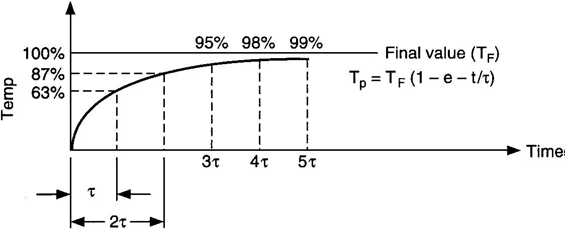
Temperature response vs. time of single capacity:
vessel-temperature lag
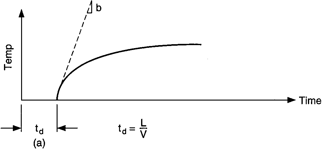
Temperature response vs. time of single capacity with dead time:
vessel-temperature lag with hot-water piping delay
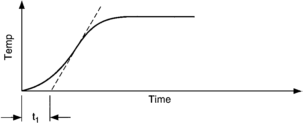
Temperature response vs. time of two capacities:
vessel-temperature lag and vessel-wall lag
Temperature response vs. time of three capacities:
vessel-temperature lag, vessel-wall lag, and thermowell-wall lag
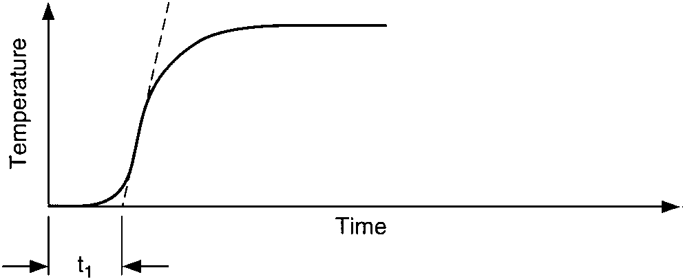
Two characteristics of these curves affect the process controllability, (1) the time interval before the temperature reaches the maximum rate of change, A, and (2) the slope of the maximum rate of change of the temperature after the change in heat input has occurred, B. The process controllability decreases as the product of A and B increases. Such increases in the product AB appear as an increasingly pronounced S-shaped curve on the graph.
The time interval A is caused by dead time, which is defined as the time between changes in heat input and the measurement of a perceptible temperature increase. The dead time includes two components, (1) propagation delay (material flow velocity delay) and (2) exponential lag (process thermal time constants).
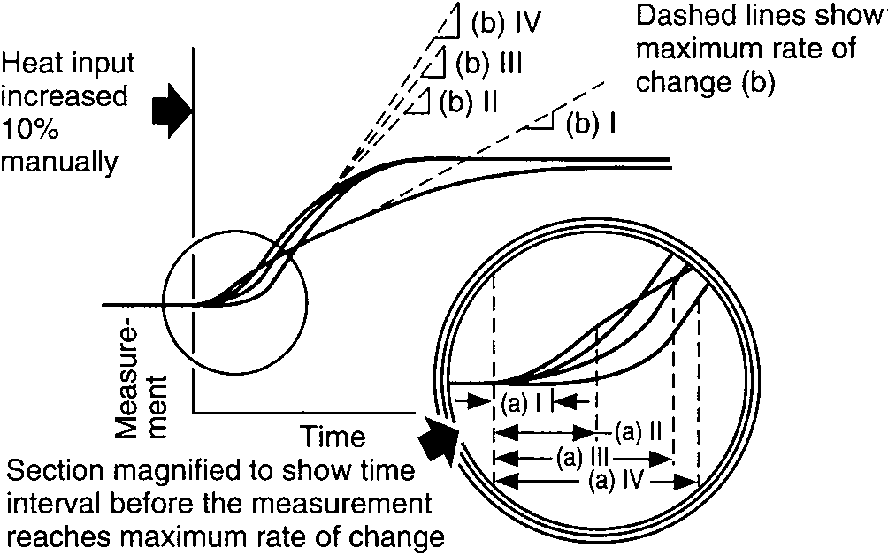
Temperature responses vs. time of temperatures I, II, III, and IV
The maximum rate of temperature rise is shown by the dashed lines which are tangent to the curves.
The tangents become progressively steeper from I to IV. The time interval before the temperature reaches the maximum rate of rise also becomes progressively greater from I to IV.
As the S curve becomes steeper, the controllability of the process becomes increasingly more difficult. As the product of the two values of time interval A and maximum rate B increases, the process controllability goes from easy (I) to very difficult (IV). Response curve IV, the most difficult process to control, has the most pronounced S shape.[1]
- Stevenson, John. “Control Principles.” Process/industrial instruments and controls handbook, 5th ed., edited by Gregory K. McMillan, McGraw-Hill, 1999, pp. 2.4-2.30.
- Shinskey, F. Greg. “Fundamentals of Process Dynamics and Control.” Perry’s chemical engineers’ handbook, 8th ed., edited by Don W. Green, McGraw-Hill, 2008, pp. 8-5 – 8-19.